NFL ML Inference Accelerator on FPGA
A football predictor that runs as a physical circuit instead of as code — two independently-trained models compiled straight into digital logic on a Basys 3, verified bit-exact from golden reference to physical board.
- Period
- Summer 2026
- Role
- Solo
- Stack
- Verilog · Python · TensorFlow/Keras · XGBoost · hls4ml · conifer · Vivado · cocotb · XSIM · pytest · Flask
- Source
- Repository
- 100 MHz
- +0.965 ns WNS, post-implementation
- 12.7K
- LUTs · 0 DSPs · 0.5 BRAM (GBDT core)
- 22
- cycle GBDT inference latency
- 100/100
- games bit-exact, golden reference to hardware
What this is
A football predictor that runs as a physical circuit instead of as code. Two models — a neural network and a gradient-boosted tree ensemble — are each trained in Python, then compiled straight into digital logic on a Basys 3’s Artix-7 and wired to a UART interface so a host application can query them live.
The project has two questions underneath it, not one: can both models be turned into working hardware, and once they are, which one is actually worth deploying — not by accuracy alone, but by what it costs in silicon.
The data and the constraint
Both models train on NFL play-by-play and game data pulled via nflreadpy across the 2000–2024
seasons, reduced to 21 feature inputs with a temporal guard — no feature is allowed to
use information from later than the game it’s predicting, which is the difference between a
model that predicts football and a model that memorizes the schedule.
The hardware constraint was fixed from the start: an Artix-7 on a Basys 3 has no floating point, no spare DSPs to assume away, and a LUT budget shared with the UART and control logic. That ruled out hand-writing either model’s RTL from scratch — instead, each model is trained in its native framework and compiled to hardware by a dedicated tool: hls4ml for the neural network, conifer for the tree ensemble.
Two models, two very different hardware costs
8-bit QAT MLP — a 128→64→32 dual-head network, 13,218 parameters, trained with quantization-aware training (not quantized after the fact) so it learns around the precision it will actually run at, with ReLU activations and MinMax-scaled inputs.
Stacked GBDT — 132 depth-2 trees for win probability and 31 depth-3 trees for spread, trained with XGBoost. The spread model predicts the residual to the Vegas line rather than a raw spread number, which turns a hard regression problem into a smaller correction on top of a strong existing baseline.
Both reach similar accuracy — ~70% test win accuracy for both, spread MAE around 9.7–9.9 for both. What separates them is what they cost once they’re actual hardware:
| GBDT | MLP | |
|---|---|---|
| LUTs | 12,095 (58%) | 17,888 (86%) |
| DSPs | 0 | 18 |
| BRAM | 0.5 | 7 |
| Inference latency | 22 cycles | 1,494 cycles |
The gap is the actual finding here, not a footnote: a decision tree is comparators and muxes, so the GBDT path uses zero DSPs and finishes in 22 cycles. The MLP’s multiply-accumulates need real multiplier hardware and a much longer pipeline. On a part this small, that difference is the whole ballgame — it’s why the GBDT core is the one wired up as the deployed design, even though the two models score almost identically.
Architecture
Data flows in a straight line and back again. The Flask UI on the host sends a game’s features over UART at 115200 baud. On the FPGA side, a UART RX/TX block with a control FSM receives them, deserializes the bytes into feature values, and hands them to whichever inference core is selected — the 8-bit QAT MLP (generated by hls4ml) or the stacked GBDT (generated by conifer). That core runs inference and produces a win probability and a spread; the control FSM streams both back over the same UART link to the host UI.
The two cores are interchangeable behind one interface: same protocol, same control FSM, same host code either way. That’s a deliberate simplification — the host never needs to know which model it’s talking to, only that it sends features and gets a prediction back.
Inside the GBDT path specifically, the two tree stages chain together through a sigmoid lookup table stored in ROM: the win-probability trees’ output feeds that table, and the result feeds the spread trees as an extra input. Around 1,300 lines of hand-written Verilog hold all of this together — the UART framing, the control FSMs, and the bidirectional host-interface logic that ties a generated core’s latency and handshake assumptions to what the protocol actually promises the host.
Verification
The standard here was zero tolerance: bit-exact agreement, not “close enough,” checked at every stage a prediction passes through, from the original Python model all the way to a physical board:
| Stage | Checked against | Tool |
|---|---|---|
| Trained model | XGBoost golden reference | pytest |
| HLS-generated core | Golden reference, in simulation | hls4ml / conifer sim |
| Post-synthesis netlist | Golden reference | XSIM |
| Physical board | Golden reference, over UART | Hardware harness |
100 out of 100 test games came back bit-exact on hardware. Zero tolerance at every earlier stage is what makes that number meaningful instead of lucky — a design that only matched “approximately” at any stage would have had nowhere to hide by the time it reached the board.
What broke, and how it was caught
- A deadlock only visible on silicon. The MLP core would hang — not in simulation, only on
the physical board. The cause was a dataflow assumption in the generated core that simulation
never stressed; the fix was forcing
hls4ml’sio_streamdataflow mode. This is exactly the class of bug the zero-tolerance-through-hardware step exists to catch: simulation had no reason to find it. - Floating-point precision mismatches. Caught by the same zero-tolerance comparison at the simulation stage, before they had a chance to become a silent, subtly-wrong hardware result.
- HLS resource estimates were off by 14× and 6.5×. The pre-synthesis area estimates from the HLS tools overstated real usage dramatically once Vivado actually synthesized and implemented the design — a reminder that an HLS tool’s own resource report is a starting estimate, not a result.
Results
Post-implementation on the Artix-7 (GBDT core, the deployed design):
| Metric | Value |
|---|---|
| Clock | 100 MHz |
| Worst negative slack | +0.965 ns |
| LUTs | 12,095 (58%) |
| DSPs | 0 |
| BRAM | 0.5 |
| Inference latency | 22 cycles |
| Win accuracy (test) | ~70.2% |
| Spread MAE (test) | ~9.76 |
| Hardware validation | 100/100 bit-exact |
+0.965 ns of slack at 100 MHz means the design isn’t scraping past timing — there’s close to a nanosecond of headroom, which is the difference between a result that reproduces and one that happens to pass this particular build.
Interactive demo
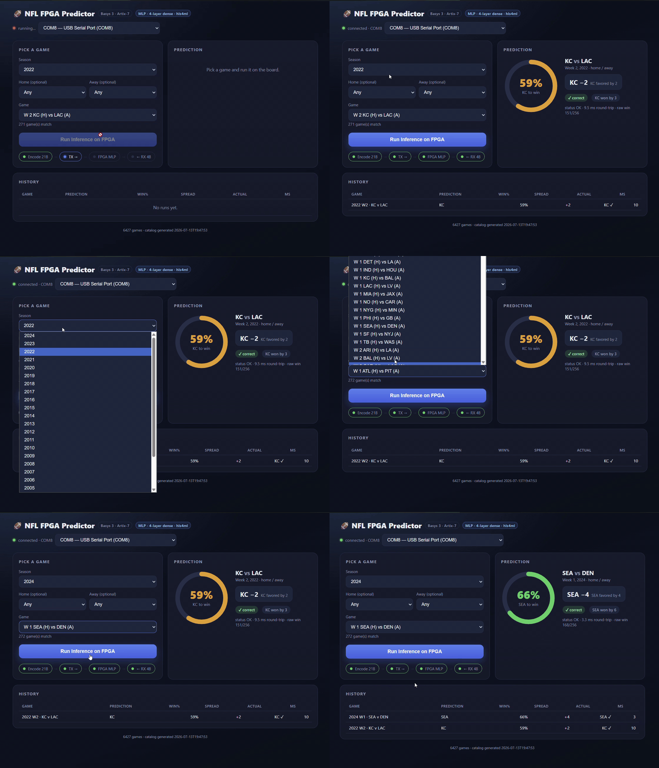
The board is wired to a Python/Flask UI that streams features down and predictions back over UART in real time, so the accelerator is something you can actually use rather than a waveform screenshot. It also turned out to be a useful debugging surface — driving real inputs by hand surfaces interface problems that structured testbenches don’t think to ask about.
What I’d do next
- Push the MLP’s latency down. 1,494 cycles against the GBDT’s 22 is the widest gap in the project; there’s real room to pipeline or restructure the MLP core before concluding the tree model simply wins on this hardware.
- Coverage, not just pass/fail. 100/100 proves the vectors I chose are correct; it doesn’t prove I chose enough of them. Constrained-random stimulus and functional coverage would replace “100/100 passed” with a defensible statement about how much of the state space was exercised.
- Wider input streaming. UART is convenient and slow relative to either inference core, which makes the link, not the math, the bottleneck.